Tao's Blog: Pearson's chi-squared test

source: http://en.wikipedia.org/wiki/Pearson%27s_chi-squared_test
Pearson's chi-squared test (χ²) is the best-known of several chi-squared tests – statistical procedures whose results are evaluated by reference to the chi-squared distribution. Its properties were first investigated by Karl Pearson in 1900.^[1] In contexts where it is important to make a distinction between the test statistic and its distribution, names similar to Pearson Χ-squared test or statistic are used.
It tests a null hypothesis stating that the frequency distribution of certain events observed in a sample is consistent with a particular theoretical distribution. The events considered must be mutually exclusive and have total probability 1. A common case for this is where the events each cover an outcome of a categorical variable. A simple example is the hypothesis that an ordinary six-sided die is "fair", i.e., all six outcomes are equally likely to occur.

Definition

Pearson's chi-squared is used to assess two types of comparison: tests of goodness of fit and tests of independence.

A test of goodness of fit establishes whether or not an observed frequency distribution differs from a theoretical distribution.
A test of independence assesses whether paired observations on two variables, expressed in a contingency table, are independent of each other—for example, whether people from different regions differ in the frequency with which they report that they support a political candidate.

The first step is to calculate the chi-squared test statistic, X², which resembles a normalized sum of squared deviations between observed and theoretical frequencies (see below). The second step is to determine the degrees of freedom, $d$ , of that statistic, which is essentially the number of frequencies reduced by the number of parameters of the fitted distribution. In the third step, X² is compared to the critical value of no significance from the $\chi^2_d$ distribution, which in many cases gives a good approximation of the distribution of X². A test that does not rely on this approximation is Fisher's exact test; it is substantially more accurate in obtaining a significance level, especially with few observations.

Test for fit of a distribution

Discrete uniform distribution

In this case $N$ observations are divided among $n$ cells. A simple application is to test the hypothesis that, in the general population, values would occur in each cell with equal frequency. The "theoretical frequency" for any cell (under the null hypothesis of a discrete uniform distribution) is thus calculated as

$E_i=\frac{N}{n}\, ,$

and the reduction in the degrees of freedom is $p=1$ , notionally because the observed frequencies $O_i$ are constrained to sum to $N$ .

Other distributions

When testing whether observations are random variables whose distribution belongs to a given family of distributions, the "theoretical frequencies" are calculated using a distribution from that family fitted in some standard way. The reduction in the degrees of freedom is calculated as $p=s+1$ , where $s$ is the number of parameters used in fitting the distribution. For instance, when checking a 3-parameter Weibull distribution, $p=4$ , and when checking a normal distribution (where the parameters are mean and standard deviation), $p=3$ . In other words, there will be $n-p$ degrees of freedom, where $n$ is the number of categories.
It should be noted that the degrees of freedom are not based on the number of observations as with a Student's t or F-distribution. For example, if testing for a fair, six-sided die, there would be five degrees of freedom because there are six categories/parameters (each number). The number of times the die is rolled will have absolutely no effect on the number of degrees of freedom.

Calculating the test-statistic

The value of the test-statistic is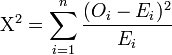

$\Chi^2 = \sum_{i=1}^{n} \frac{(O_i - E_i)^2}{E_i}$

where

$\Chi^2$ = Pearson's cumulative test statistic, which asymptotically approaches a $\chi^2$ distribution.

$O_i$ = an observed frequency;

$E_i$ = an expected (theoretical) frequency, asserted by the null hypothesis;

$n$ = the number of cells in the table.

Chi-squared distribution, showing X² on the x-axis and P-value on the y-axis.

The chi-squared statistic can then be used to calculate a p-value by comparing the value of the statistic to a chi-squared distribution. The number of degrees of freedom is equal to the number of cells $n$ , minus the reduction in degrees of freedom, $p$ .
The result about the number of degrees of freedom is valid when the original data was multinomial and hence the estimated parameters are efficient for minimizing the chi-squared statistic. More generally however, when maximum likelihood estimation does not coincide with minimum chi-squared estimation, the distribution will lie somewhere between a chi-squared distribution with $n-1-p$ and $n-1$ degrees of freedom (See for instance Chernoff and Lehmann, 1954).

Bayesian method

For more details on this topic, see Categorical distribution#Bayesian statistics.

In Bayesian statistics, one would instead use a Dirichlet distribution as conjugate prior. If one took a uniform prior, then the maximum likelihood estimate for the population probability is the observed probability, and one may compute a credible region around this or another estimate.

Test of independence

In this case, an "observation" consists of the values of two outcomes and the null hypothesis is that the occurrence of these outcomes is statistically independent. Each observation is allocated to one cell of a two-dimensional array of cells (called a table) according to the values of the two outcomes. If there are r rows and c columns in the table, the "theoretical frequency" for a cell, given the hypothesis of independence, is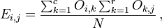

$E_{i,j}=\frac{\sum_{k=1}^c O_{i,k} \sum_{k=1}^r O_{k,j}}{N} \, ,$

where N is the total sample size (the sum of all cells in the table). The value of the test-statistic is

$\Chi^2 = \sum_{i=1}^{r} \sum_{j=1}^{c} {(O_{i,j} - E_{i,j})^2 \over E_{i,j}} .$

Fitting the model of "independence" reduces the number of degrees of freedom by p = r + c − 1. The number of degrees of freedom is equal to the number of cells rc, minus the reduction in degrees of freedom, p, which reduces to (r − 1)(c − 1).
For the test of independence, also known as the test of homogeneity, a chi-squared probability of less than or equal to 0.05 (or the chi-squared statistic being at or larger than the 0.05 critical point) is commonly interpreted by applied workers as justification for rejecting the null hypothesis that the row variable is independent of the column variable.^[2] The alternative hypothesis corresponds to the variables having an association or relationship where the structure of this relationship is not specified.

Tao's Blog

Wednesday 7 March 2012

Pearson's chi-squared test