Sunday 27 May 2012

Working Log May 25

Goal:
New Task reviewing.
Intensive text processing by mapreduce reading.

Thursday 24 May 2012

Task and Goal:

1. Read the perl best practice, optimize recently code fallow the conventions learned from the book.

2. Finalise the Duplicate Analysis and write analysis.

3. Getting new tasks and reading plan.

What have been Done:
1. A better look at Perl variables, without a explicitly declaration, the scope is package wide, with my it's local, always use local as it is.

Review:
1. Done
2. Done Beautifully
3. check grep function
4. Large text processing using mapreduce to 3.1
5. Should have use combiners to optimize my mapreduce programs

Thursday 12 April 2012

Working Log April 12

A power law is a special kind of mathematical relationship between two quantities. When the frequency of an event varies as a power of some attribute of that event (e.g. its size), the frequency is said to follow a power law. For instance, the number of cities having a certain population size is found to vary as a power of the size of the population, and hence follows a power law. There is evidence that the distributions of a wide variety of physical, biological, and man-made phenomena follow a power law, including the sizes of earthquakes, craters on the moon and of solar flares,^[1] the foraging pattern of various species,^[2] the sizes of activity patterns of neuronal populations,^[3] the frequencies of words in most languages, frequencies of family names, the species richness in clades of organisms,^[4] the sizes of power outages and wars,^[5] and many other quantities.

K-Means Clustering Overview

Overview

K-Means clustering generates a specific number of disjoint, flat (non-hierarchical) clusters. It is well suited to generating globular clusters. The K-Means method is numerical, unsupervised, non-deterministic and iterative.

K-Means Algorithm Properties

There are always K clusters.
There is always at least one item in each cluster.
The clusters are non-hierarchical and they do not overlap.
Every member of a cluster is closer to its cluster than any other cluster because closeness does not always involve the 'center' of clusters.

The K-Means Algorithm Process

The dataset is partitioned into K clusters and the data points are randomly assigned to the clusters resulting in clusters that have roughly the same number of data points.
For each data point:
Calculate the distance from the data point to each cluster.
If the data point is closest to its own cluster, leave it where it is. If the data point is not closest to its own cluster, move it into the closest cluster.
Repeat the above step until a complete pass through all the data points results in no data point moving from one cluster to another. At this point the clusters are stable and the clustering process ends.
The choice of initial partition can greatly affect the final clusters that result, in terms of inter-cluster and intracluster distances and cohesion.

K-Means Clustering in GeneLinker™

The version of the K-Means algorithm used in GeneLinker™ differs from the conventional K-Means algorithm in that GeneLinker™ does not compute the centroid of the clusters to measure the distance from a data point to a cluster. Instead, the algorithm uses a specified linkage distance metric. The use of the Average Linkage distance metric most closely corresponds to conventional K-Means, but can produce different results in many cases.

Advantages to Using this Technique

With a large number of variables, K-Means may be computationally faster than hierarchical clustering (if K is small).
K-Means may produce tighter clusters than hierarchical clustering, especially if the clusters are globular.

Disadvantages to Using this Technique

Difficulty in comparing quality of the clusters produced (e.g. for different initial partitions or values of K affect outcome).
Fixed number of clusters can make it difficult to predict what K should be.
Does not work well with non-globular clusters.
Different initial partitions can result in different final clusters. It is helpful to rerun the program using the same as well as different K values, to compare the results achieved.

The Euclidean distance between points p and q is the length of the line segment connecting them ( $\overline{\mathbf{p}\mathbf{q}}$ ).
In Cartesian coordinates, if p = (p₁, p₂,..., p_n) and q = (q₁, q₂,..., q_n) are two points in Euclidean n-space, then the distance from p to q, or from q to p is given by

$\mathrm{d}(\mathbf{p},\mathbf{q}) = \mathrm{d}(\mathbf{q},\mathbf{p}) = \sqrt{(q_1-p_1)^2 + (q_2-p_2)^2 + \cdots + (q_n-p_n)^2} = \sqrt{\sum_{i=1}^n (q_i-p_i)^2}.$

Tuesday 27 March 2012

Hadoop Debugging Notes

Today, when running a mapreduce job on 4 Amazon m1.xlarge nodes. Got the fallowing error.

java.io.IOException: Cannot run program "bash": java.io.IOException: error=12, Cannot allocate memory

java.lang.Throwable: Child Error
at org.apache.hadoop.mapred.TaskRunner.run(TaskRunner.java:532)

As amazon instance doesn't provide any swap space which means all the process are stay fully in memory all the time. It's very easy to cause memory problems. TO solve the above errors. Simply add swap space in your amazon instance.

Another course could be overload nodes, it's very important to have a proper task numbers, overloaded nodes may lead to memory problems too.

A Glance at the Hadoop Failure Model

By nathan marz | Published: July 17, 2009

Hadoop is designed to be a fault tolerant system. Jobs should be resilient to nodes going down and other random failures. Hadoop isn’t perfect however, as I still see jobs failing due to random causes every now and again. I decided to investigate the significance of the different factors that play into a job failing.
A Hadoop job fails if the same task fails some predetermined amount of times (by default, four). This is set through the properties “mapred.map.max.attempts” and “mapred.reduce.max.attempts”. For a job to fail randomly, an individual task will need to fail randomly this predetermined amount of times. A task can fail randomly for a variety of reasons – a few of the ones we’ve seen are disks getting full, a variety of bugs in Hadoop, and hardware failures.
The formula for the probability of a job failing randomly can be derived as follows:



Pr[individual task failing maximum #times] = Pr[task failing] ^ (max task failures)

Pr[task succeeding] = 1 - Pr[individual task failing maximum #times]

Pr[job succeeding] = Pr[task succeeding] ^ (num tasks)

Pr[job failing] = 1 - Pr[job succeeding]

Pr[job failing] = 1 - (1-Pr[task failing] ^ (max task failures))^(num tasks)

The maximum amount of task failures is set through the property “mapred.max.tracker.failures” and defaults to 4.
Let’s take a significant workload of 100,000 map tasks and see what the numbers look like:

As the probability of a task failing goes above 1%, the probability of the job failing rapidly increases. It is very important to keep the cluster stable and keep the failure rate relatively small, as these numbers show Hadoop’s failure model only goes so far. We can also see the importance of the “max task failures” parameter, as values under 4 cause the probability of job failures to rise to significant values even with a 0.5% probability of task failure.
Reducers run for a much longer period of time than mappers, which means a reducer has more time for a random event to cause it to fail. We can therefore say that the probability of a reducer failing is much higher than a mapper failing. This is balanced out by the fact that there are a much smaller amount of reducers. Let’s look at some numbers more representative of a job failing due to reducers failing:

The probabilities of a reducer failing need to go up to 10% to have a significant chance of failure.

Bad Nodes

One more variable to consider in the model is bad nodes. Oftentimes nodes go bad and every task run on them fails, whether because of a disk going bad, the disk filling up, or other causes. With a bad node, you typically see a handful of mappers and reducers fail before the node gets blacklisted and no more tasks are assigned to it. In order to simplify our analysis, let’s assume that each bad node causes a fixed number of tasks to fail. Additionally, let’s assume a task can only be affected by a bad node once, which is reasonable because nodes are blacklisted fairly quickly. Let’s call the tasks which fail once due to a bad node “b-tasks” and the other tasks “n-tasks”. A “b-task” starts with one failure, so it needs to fail randomly “max task failures – 1″ times to cause the job to fail. On our cluster, we typically see a bad node cause three tasks to automatically fail, so using that number the modified formula ends up looking like:



#b-tasks = #bad nodes * 3

Pr[all b-tasks succeeding] = (1-Pr[task failing] ^ (max task failures - 1))^(#b-tasks)

Pr[all n-tasks succeeding] =  (1-Pr[task failing] ^ (max task failures))^(num tasks - #b-tasks)

Pr[job succeeding] = Pr[all b-tasks succeeding] * Pr[all n-tasks succeeding]

Pr[job succeeding] = (1-Pr[task failing] ^ (max task failures - 
1))^(#b-tasks) * (1-Pr[task failing] ^ (max task failures))^(num tasks -
 #b-tasks)

Pr[job failing] = 1 - Pr[job succeeding]

Pr[job failing] = 1 - (1-Pr[task failing] ^ (max task failures - 1))^(#b-tasks) * (1-Pr[task failing] ^ (max task failures))^(num tasks - #b-tasks)

Since there are so many mappers, the results of the formula won’t change for a handful of bad nodes. Given that the number of reducers is relatively small though, the numbers do change somewhat:

Happily the numbers aren’t too drastic – five bad nodes causes the failure rate to increase by 1.5x to 2x.
In the end, Hadoop is fairly fault tolerant as long as the probability of a task failing is kept relatively low. Based on the numbers we’ve looked at, 4 is a good value to use for “max task failures”, and you should start worrying about cluster stability when the task failure rate approaches 1%. You could always increase the “max task failures” properties to increase robustness, but if you are having that many failures you will be suffering performance penalties and would be better off making your cluster more stable.

Saturday 10 March 2012

Rails study notes 1

Rails as as MVC fraework
model view controller
controller(models.rb) rails routing

1. Routes map incoming url's to controller actions
2. controller actions set instance vairables, visible to views
3. controller action enventually renders a view

Convention over configuration: if naming follows certain conventions, no need for config files
Don't repear yourself: mechanisms to exract common functionality

Database:
Rails feature:
Testing: develpment and production and test enviroments each have own DB
Mirgration: scripts to descripe the change

up version and down version of migration methods, that makes everything reversible
Apply migration to development:
rake db:migrate

Add a new model
rails generate migration

Raisl generate sql statement at runtime, based on ruby code

Subclassing from ActiveRecord::Base
connects a model to a database

Reading things in the database
Movie.where("rating = 'PG')

Add a action
1. create route in config/routes.rb
2. Add the action in the apporcatia place
3. add the view coresspondinly

Debug
Printing to termial
log file

when debugging, the error information can be very useful, the information could tell us where th error is in the ruby.
Don't use puts or printf to print error message, as they may just been print out on the terminal, and the information will lost forever

Wednesday 7 March 2012

Pearson's chi-squared test

source: http://en.wikipedia.org/wiki/Pearson%27s_chi-squared_test
Pearson's chi-squared test (χ²) is the best-known of several chi-squared tests – statistical procedures whose results are evaluated by reference to the chi-squared distribution. Its properties were first investigated by Karl Pearson in 1900.^[1] In contexts where it is important to make a distinction between the test statistic and its distribution, names similar to Pearson Χ-squared test or statistic are used.
It tests a null hypothesis stating that the frequency distribution of certain events observed in a sample is consistent with a particular theoretical distribution. The events considered must be mutually exclusive and have total probability 1. A common case for this is where the events each cover an outcome of a categorical variable. A simple example is the hypothesis that an ordinary six-sided die is "fair", i.e., all six outcomes are equally likely to occur.

Definition

Pearson's chi-squared is used to assess two types of comparison: tests of goodness of fit and tests of independence.

A test of goodness of fit establishes whether or not an observed frequency distribution differs from a theoretical distribution.
A test of independence assesses whether paired observations on two variables, expressed in a contingency table, are independent of each other—for example, whether people from different regions differ in the frequency with which they report that they support a political candidate.

The first step is to calculate the chi-squared test statistic, X², which resembles a normalized sum of squared deviations between observed and theoretical frequencies (see below). The second step is to determine the degrees of freedom, $d$ , of that statistic, which is essentially the number of frequencies reduced by the number of parameters of the fitted distribution. In the third step, X² is compared to the critical value of no significance from the $\chi^2_d$ distribution, which in many cases gives a good approximation of the distribution of X². A test that does not rely on this approximation is Fisher's exact test; it is substantially more accurate in obtaining a significance level, especially with few observations.

Test for fit of a distribution

Discrete uniform distribution

In this case $N$ observations are divided among $n$ cells. A simple application is to test the hypothesis that, in the general population, values would occur in each cell with equal frequency. The "theoretical frequency" for any cell (under the null hypothesis of a discrete uniform distribution) is thus calculated as

$E_i=\frac{N}{n}\, ,$

and the reduction in the degrees of freedom is $p=1$ , notionally because the observed frequencies $O_i$ are constrained to sum to $N$ .

Other distributions

When testing whether observations are random variables whose distribution belongs to a given family of distributions, the "theoretical frequencies" are calculated using a distribution from that family fitted in some standard way. The reduction in the degrees of freedom is calculated as $p=s+1$ , where $s$ is the number of parameters used in fitting the distribution. For instance, when checking a 3-parameter Weibull distribution, $p=4$ , and when checking a normal distribution (where the parameters are mean and standard deviation), $p=3$ . In other words, there will be $n-p$ degrees of freedom, where $n$ is the number of categories.
It should be noted that the degrees of freedom are not based on the number of observations as with a Student's t or F-distribution. For example, if testing for a fair, six-sided die, there would be five degrees of freedom because there are six categories/parameters (each number). The number of times the die is rolled will have absolutely no effect on the number of degrees of freedom.

Calculating the test-statistic

The value of the test-statistic is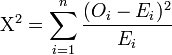

$\Chi^2 = \sum_{i=1}^{n} \frac{(O_i - E_i)^2}{E_i}$

where

$\Chi^2$ = Pearson's cumulative test statistic, which asymptotically approaches a $\chi^2$ distribution.

$O_i$ = an observed frequency;

$E_i$ = an expected (theoretical) frequency, asserted by the null hypothesis;

$n$ = the number of cells in the table.

Chi-squared distribution, showing X² on the x-axis and P-value on the y-axis.

The chi-squared statistic can then be used to calculate a p-value by comparing the value of the statistic to a chi-squared distribution. The number of degrees of freedom is equal to the number of cells $n$ , minus the reduction in degrees of freedom, $p$ .
The result about the number of degrees of freedom is valid when the original data was multinomial and hence the estimated parameters are efficient for minimizing the chi-squared statistic. More generally however, when maximum likelihood estimation does not coincide with minimum chi-squared estimation, the distribution will lie somewhere between a chi-squared distribution with $n-1-p$ and $n-1$ degrees of freedom (See for instance Chernoff and Lehmann, 1954).

Bayesian method

For more details on this topic, see Categorical distribution#Bayesian statistics.

In Bayesian statistics, one would instead use a Dirichlet distribution as conjugate prior. If one took a uniform prior, then the maximum likelihood estimate for the population probability is the observed probability, and one may compute a credible region around this or another estimate.

Test of independence

In this case, an "observation" consists of the values of two outcomes and the null hypothesis is that the occurrence of these outcomes is statistically independent. Each observation is allocated to one cell of a two-dimensional array of cells (called a table) according to the values of the two outcomes. If there are r rows and c columns in the table, the "theoretical frequency" for a cell, given the hypothesis of independence, is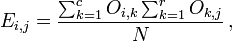

$E_{i,j}=\frac{\sum_{k=1}^c O_{i,k} \sum_{k=1}^r O_{k,j}}{N} \, ,$

where N is the total sample size (the sum of all cells in the table). The value of the test-statistic is

$\Chi^2 = \sum_{i=1}^{r} \sum_{j=1}^{c} {(O_{i,j} - E_{i,j})^2 \over E_{i,j}} .$

Fitting the model of "independence" reduces the number of degrees of freedom by p = r + c − 1. The number of degrees of freedom is equal to the number of cells rc, minus the reduction in degrees of freedom, p, which reduces to (r − 1)(c − 1).
For the test of independence, also known as the test of homogeneity, a chi-squared probability of less than or equal to 0.05 (or the chi-squared statistic being at or larger than the 0.05 critical point) is commonly interpreted by applied workers as justification for rejecting the null hypothesis that the row variable is independent of the column variable.^[2] The alternative hypothesis corresponds to the variables having an association or relationship where the structure of this relationship is not specified.

Work Log Mar 6

1. Unix Command
pushd and popd
The pushd command saves the current working directory in memory so it can be returned to at any time, optionally changing to a new directory. The popd command returns to the path at the top of the directory stack.

Tuesday 28 February 2012

Working log

Working Log
1. Verify the compression ratio of a web page

The compression ratio is majorly used to detect the repeated words in a web page, here define compression ratio of a web page is the uncompressed page divided by the compressed page, therefore, the higher the compression ratio is, it is more likely to be a spam page.

2. Verify the n-gram liklyhoods

Many spam page may generate content by drawn words randomly from a dictionary.

3. Anchor fraction
Some search engine take the anchor text as a keyword to the link in the anchor, so some spam page are created to major for creating the keyword for other sites.
So the anchor fraction could indicate the spamicity of a cite.

Tao's Blog

Sunday 27 May 2012

Working Log May 25

Thursday 24 May 2012

Working Log May 24

Thursday 12 April 2012

Working Log April 12

K-Means Clustering Overview

Tuesday 27 March 2012

Hadoop Debugging Notes

A Glance at the Hadoop Failure Model

A Glance at the Hadoop Failure Model

Bad Nodes

Saturday 10 March 2012

Rails study notes 1

Wednesday 7 March 2012

Pearson's chi-squared test

Definition

Test for fit of a distribution

Discrete uniform distribution

Other distributions

Calculating the test-statistic

Bayesian method

Test of independence

Work Log Mar 6

Tuesday 28 February 2012

Working log